Example Fit
As a semi-analytical model, SALT is designed to compute spectral lines quickly. When paired with a Monte Carlo sampler, one can constrain the SALT parameter space efficently to determine the properties of galactic outflows and the associated uncertainties. In this tutorial, we fit SALT to the spectrum of a real galaxy using the Python based Markov Chain Monte Carlo (MCMC) ensemble sampler, emcee (Foreman-Mackey, Hogg, Lang & Goodman 2012). The goal is to sufficiently sample a likelihood function to quantify the best parameter fit and associated uncertainties. For this tutorial, we assume a Gaussian likelihood function. The fitting code is described below.
Fitting with MCMC
import numpy as np
import scipy.ndimage.filters as g
from scipy import interpolate
import emcee
import corner
#import sys
#sys.path.insert(0, 'path')
from SALT2022_LineProfile import Line_Profile

# rebin data
def rebin(x,y,xnew):
   f = interpolate.interp1d(x,y)
   ynew = f(xnew)
   return ynew

# likelihood
def lnlike(pars, y, yerr):

   # SALT parameters
   alpha,psi,gamma, tau, v_0, v_w, f_c, k, delta, v_ap = pars

   tau = 10.0**tau
   k = 10.0**k
   delta = gamma+2.0+delta

   background = np.ones_like(v_range)

   OCCULTATION = True
   APERTURE = True

   profile_type = 'pcygni'

   flow_parameters = {'alpha':alpha, 'psi':psi, 'gamma':gamma, 'tau':tau, 'v_0':v_0, 'v_w':v_w, 'v_ap':v_ap, 'f_c':f_c, 'k':k, 'delta':delta}
   profile_parameters = {'abs_waves':[1190.42,1193.28],'abs_osc_strs':[0.277,.575], 'em_waves':[1190.42,1190.42,1193.28,1193.28],'em_osc_strs':[0.277,0.277,0.575,0.575],'res':[True,False,True,False],'fluor':[False,True,False,True],'p_r':[.1592,.1592,.6577,.6577],'p_f':[.8408,.8408,.3423,.3423],'final_waves':[1190.42,1194.5,1193.28,1197.39],'line_num':[2,2], 'v_obs':v_range,'lam_ref':lam_ref, 'APERTURE':APERTURE,'OCCULTATION':OCCULTATION}

   # SALT is first run on a higher resolution array, then smoothed and rebinned to match the data
   model = Line_Profile(v_range,lam_ref,background,flow_parameters,profile_parameters,profile_type)
   model = np.array(g.gaussian_filter1d(model,res))
   model = rebin(v_range,model,v_obs)

   # log Gaussian likelihood
   result = 0
   for i in range(len(list(y))):
      sigma = 1.0/yerr[i]**2.0
      result += (((y[i]-model[i])**2.0*sigma)-np.log(sigma))
   result = -.5*result
   return result

# prior probability
def lnprior(pars):
   alpha,psi,gamma,tau,v_0,v_w,f_c,k,delta,v_ap = pars
   if 0<alpha<np.pi/2.0 and 0<psi<np.pi/2.0 and 0.5<gamma<2.0 and -2<tau<3 and 2.0<v_0<150.0 and 200.0<v_w<1500.0 and 0<f_c<1 and -2.0<k<2.0 and -1.5<delta<1.5 and 0<v_ap<1500:
      return 0
   return -np.Inf

# full probability
def lnprob(pars,y,yerr):
   lnp = lnprior(pars)
   if not np.isfinite(lnp):
      return -np.Inf
   return lnp + lnlike(pars,y,yerr)

# run emcee
def main():
   sampler = emcee.EnsembleSampler(nwalkers, ndim, lnprob, args=(np.array(flux), np.array(error)), pool=Pool(max_workers = 25))
   start_time = time.time()
   sampler.run_mcmc(p0, steps);
   print("--- %s seconds ---" % (time.time() - start_time))
   np.savetxt('chain_pars.txt',sampler.chain.reshape((-1, ndim)))
   np.savetxt('max_likelihood_pars.txt',sampler.get_log_prob().reshape((-1, nwalkers)))

# get data to fit
data = np.loadtxt('0911+1831.txt')
v_obs = data[:,0]
flux = data[:,1]
error = data[:,2]

# SALT is first run on a higher resolution array, then smoothed and rebinned to match data
lam_ref = 1193.28
v_range = np.linspace(-2500,2500,1500)
res = 30.0/(v_range[1]-v_range[0])

# randomly generates initial conditions
ndim, nwalkers, steps = 10, 50, 3000
p0 = np.random.rand(nwalkers,ndim)

p0[:,0] = p0[:,0] * np.pi/2.0
p0[:,1] = p0[:,1] * np.pi/2.0
p0[:,2] = p0[:,2] * 1.5+.5
p0[:,3] = p0[:,3] * 5.0-2.0
p0[:,4] = p0[:,4] * 98. +2.
p0[:,5] = p0[:,5] * 600.0+200.0
p0[:,6] = p0[:,6]
p0[:,7] = p0[:,7] * 4.0-2.0
p0[:,8] = p0[:,8] * 3.0-1.5
p0[:,9] = p0[:,9] * 600.0+200.0

if __name__ == "__main__":
   main()
Results
Here we analyize the results of the model fitting.
import numpy as np
import scipy.ndimage.filters as g
from scipy import interpolate
from matplotlib import pyplot as plt
from SALT2022_LineProfile import Line_Profile
def rebin(x,y,xnew):
f = interpolate.interp1d(x,y)
ynew = f(xnew)
return ynew
# get data
data = np.loadtxt('0911+1831.txt')
v_obs = data[:,0]
flux = data[:,1]
error = data[:,2]
eu = flux+error
ed = flux-error
# get chains
chain = np.genfromtxt('0911_chains.txt')
ndim, nwalkers, steps = 10, 50, 3000
chain = np.reshape(chain,(nwalkers,steps,ndim))
# collect chains
alpha_chain = chain[:,:,0]
psi_chain = chain[:,:,1]
gamma_chain = chain[:,:,2]
tau_chain = 10.0**chain[:,:,3]
v_0_chain = chain[:,:,4]
v_w_chain = chain[:,:,5]
f_c_chain = chain[:,:,6]
k_chain = 10.0**chain[:,:,7]
delta_chain = chain[:,:,8]+chain[:,:,2]+2.0
v_ap_chain = chain[:,:,9]
# find best fit from likelihood samples
likelihood = np.genfromtxt('0911_likelihoods.txt').ravel()
bf_index = np.where(likelihood == max(likelihood))[0][0]
f1=int(bf_index%nwalkers)
f2=int((bf_index-f1)/nwalkers)
# best fit SALT parameters
alpha = chain[f1,f2,0]
psi = chain[f1,f2,1]
gamma = chain[f1,f2,2]
tau = 10**chain[f1,f2,3]
v_0 = chain[f1,f2,4]
v_w = chain[f1,f2,5]
f_c = chain[f1,f2,6]
k = 10**chain[f1,f2,7]
delta = chain[f1,f2,8]+chain[f1,f2,2]+2.0
v_ap= chain[f1,f2,9]
# compute SALT
lam_ref = 1193.28
v_range = np.linspace(int(v_obs[0])-1.0,int(v_obs[-1])+1,1500)
background = np.ones_like(v_range)
OCCULTATION = True
APERTURE = True
profile_type = 'pcygni'
flow_parameters = {'alpha':alpha, 'psi':psi, 'gamma':gamma, 'tau':tau, 'v_0':v_0, 'v_w':v_w, 'v_ap':v_ap, 'f_c':f_c, 'k':k, 'delta':delta}
profile_parameters = {'abs_waves':[1190.42,1193.28],'abs_osc_strs':[0.277,.575], 'em_waves':[1190.42,1190.42,1193.28,1193.28],'em_osc_strs':[0.277,0.277,0.575,0.575],'res':[True,False,True,False],'fluor':[False,True,False,True],'p_r':[.1592,.1592,.6577,.6577],'p_f':[.8408,.8408,.3423,.3423],'final_waves':[1190.42,1194.5,1193.28,1197.39],'line_num':[2,2], 'v_obs':v_range,'lam_ref':lam_ref, 'APERTURE':APERTURE,'OCCULTATION':OCCULTATION}
spectrum = Line_Profile(v_range,lam_ref,background,flow_parameters,profile_parameters,profile_type)
# smooth and rebin data
res = 30.0/(v_range[1]-v_range[0])
spectrum = np.array(g.gaussian_filter1d(spectrum,res))
spectrum = rebin(v_range,spectrum,v_obs)
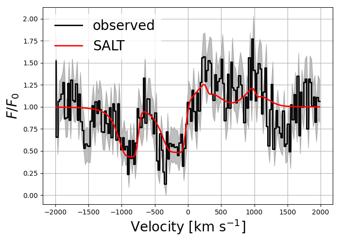
from matplotlib import pyplot as plt
fig, ax = plt.subplots(1,1, figsize=(7, 5))
ax.fill_between(v_obs, eu, ed,alpha = .5,color = 'grey')
ax.step(v_obs,flux,'k',linewidth = 2,label='observed')
ax.plot(v_obs,spectrum,'r',linewidth = 2.0,label='SALT')
ax.set_xlabel('Velocity '+r'$[\rm km \ s^{-1}]$',fontsize =20)
ax.set_ylabel(r'$F/F_0$',fontsize =20)
ax.legend(loc='upper left',fontsize = 20,edgecolor = 'white',facecolor = 'white',framealpha=0.8)
plt.grid()
plt.tight_layout()
plt.show()
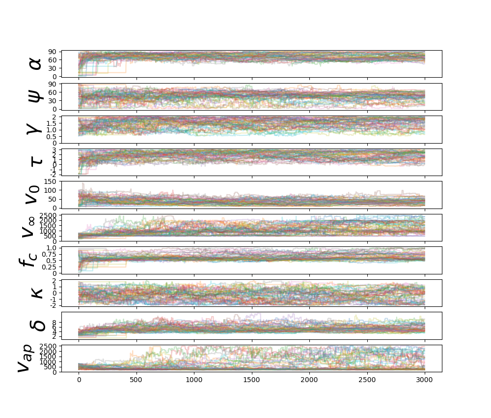
# show steps in parameter space
fig,(ax1,ax2,ax3,ax4,ax5,ax6,ax7,ax8,ax9,ax10) = plt.subplots(10,1,figsize=(10,8.5))

ax1.plot((180/np.pi)*alpha_chain.T,alpha=0.25)
ax2.plot((180/np.pi)*psi_chain.T,alpha=0.25)
ax3.plot(gamma_chain.T,alpha=0.25)
ax4.plot(tau_chain.T,alpha=0.25)
ax5.plot(v_0_chain.T,alpha=0.25)
ax6.plot(v_w_chain.T,alpha=0.25)
ax7.plot(f_c_chain.T,alpha=0.25)
ax8.plot(k_chain.T,alpha=0.25)
ax9.plot(delta_chain.T,alpha=0.25)
ax10.plot(v_ap_chain.T,alpha=0.25)

# alpha
ax1.set_yticks([0,30,60,90])
ax1.set_yticklabels([0,30,60,90])
ax1.set_xticklabels([])

# psi
ax2.set_yticks([0,30,60,90])
ax2.set_yticklabels([0,30,60,90])
ax2.set_xticklabels([])

# gamma
ax3.set_yticks([0,0.5,1.0,1.5,2])
ax3.set_yticklabels([0,0.5,1.0,1.5,2])
ax3.set_xticklabels([])

# tau
ax4.set_yticks([-2,-1,0,1,2,3])
ax4.set_yticklabels([-2,-1,0,1,2,3])
ax4.set_xticklabels([])

# v_0
ax5.set_yticks([0,50,100,150])
ax5.set_yticklabels([0,50,100,150])
ax5.set_xticklabels([])

# v_w
ax6.set_yticks([0,500,1000,1500,2000,2500])
ax6.set_yticklabels([0,500,1000,1500,2000,2500])
ax6.set_xticklabels([])

# f_c
ax7.set_yticks([0,.25,.5,.75,1])
ax7.set_yticklabels([0,0.25,0.5,0.75,1.0])
ax7.set_xticklabels([])

# kappa
ax8.set_yticks([-2,-1,0,1,2])
ax8.set_yticklabels([-2,-1,0,1,2])
ax8.set_xticklabels([])

# delta
ax9.set_yticks([2,4,6,8])
ax9.set_yticklabels([2,4,6,8])
ax9.set_xticklabels([])

# v_ap
ax10.set_yticks([0,500,1000,1500,2000,2500])
ax10.set_yticklabels([0,500,1000,1500,2000,2500])

ax1.set_ylabel(r'$\alpha$',fontsize = 30)
ax2.set_ylabel(r'$\psi$',fontsize = 30)
ax3.set_ylabel(r'$\gamma$',fontsize = 30)
ax4.set_ylabel(r'$\tau$',fontsize = 30)
ax5.set_ylabel(r'$v_0$',fontsize = 30)
ax6.set_ylabel(r'$v_{\infty}$',fontsize = 30)
ax7.set_ylabel(r'$f_c$',fontsize = 30)
ax8.set_ylabel(r'$\kappa$',fontsize = 30)
ax9.set_ylabel(r'$\delta$',fontsize = 30)
ax10.set_ylabel(r'$v_{ap}$',fontsize = 30)

for ax in [ax1,ax2,ax3,ax4,ax5,ax6,ax7,ax8,ax9]:
   ax.set_xlabel('Number of Steps',fontsize = 30)
   fig = plt.gcf()
plt.show()
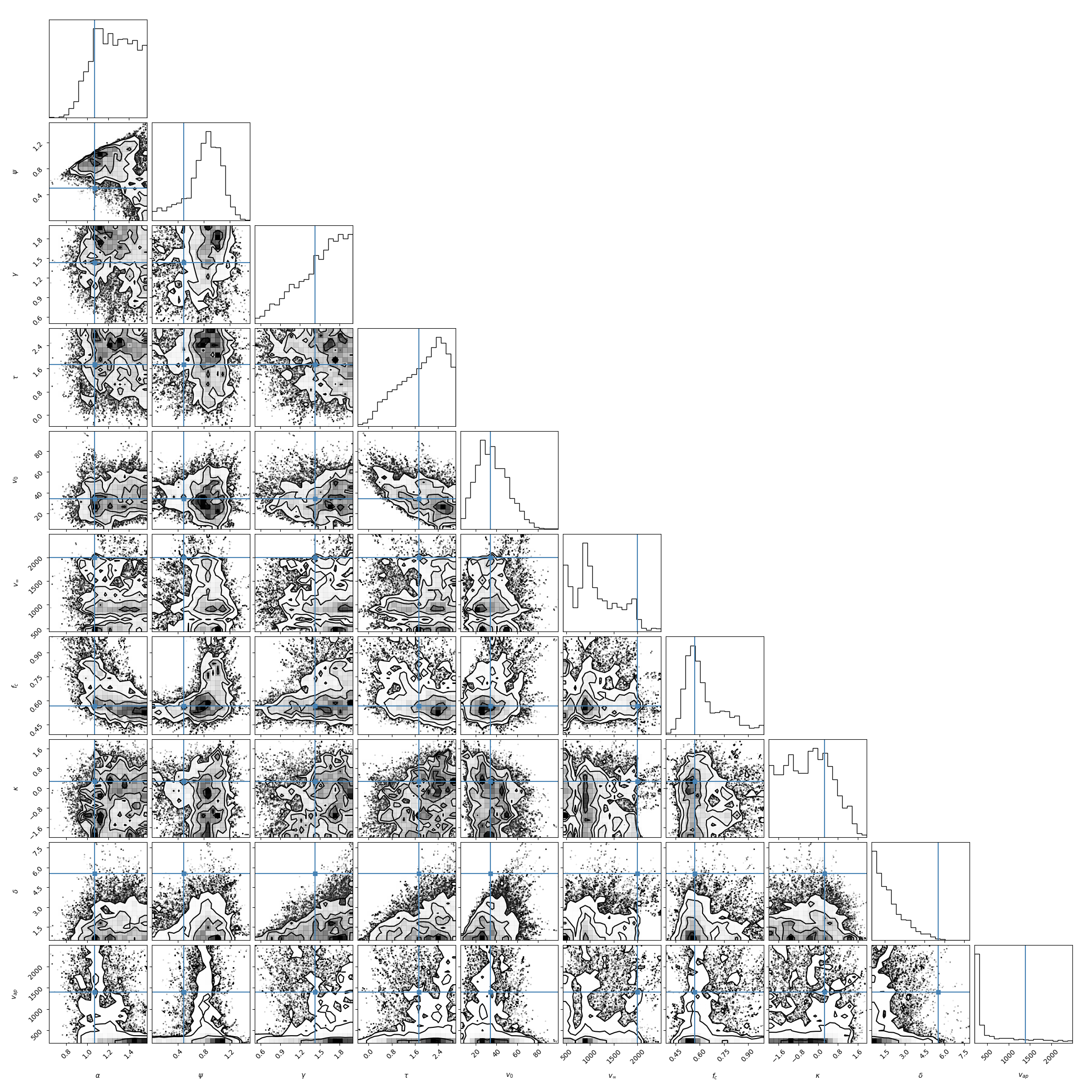
# marginal pdfs, removed 'burning phase', best fit shown in blue
import corner
samples = chain[:,500:,:].reshape((-1, ndim))
fig = corner.corner(samples, labels=[r'$\alpha$',r'$\psi$',r'$\gamma$',r'$\tau$',r'$v_0$',r'$v_{\infty}$',r'$f_c$',r'$\kappa$',r'$\delta$',r'$v_{ap}$'],truths=[alpha, psi, gamma, tau, v_0, v_w, f_c, k, delta, v_ap])
fig.savefig("pdfs.png")